Chapter 5 Ggplot and dplyr
Learning Objectives:
In this chapter, we will master the art of data storytelling. We will learn to create layered visualizations using ggplot2, customizing every aspect from aesthetics and scales to themes and labels. Additionally, we will gain proficiency in summarizing data with dplyr functions like summarize() and group_by(), all while deepening our understanding of the grammar of graphics approach.
Building on the basic plotting skills from previous chapters, we’ll now create more sophisticated and visually polished visualizations. The ggplot2 package provides a powerful and consistent framework for building graphics layer by layer.
To get started, we’ll use the ggplot object included in the tidyverse library (the tidyverse package includes ggplot2 among its core packages). Since we’ve already installed tidyverse previously, we only need to load it:
We’ll learn these visualization techniques using our previous case/problem, allowing us to build up our ggplot skills gradually with familiar data.
5.1 Creating the ggplot object
We will start by creating the ggplot object from the murders data using the pipeline operator |>. Let’s also remember to have loaded the murders data from the dslabs library.

This code only shows us an empty box. This is because we haven’t specified which variables to take from the data frame nor what type of plot we want.
To build our plot, we’ll add components using layers. The ggplot system allows us to add one layer at a time, each specifying a different aspect of the visualization. We connect layers using the + operator.
5.2 Aesthetic mapping layer
First we will focus on the basic aesthetics, that is: what goes on the x-axis and what we put on the y-axis. To do this we will use the aesthetic function which in R is aes(). For example, let’s add the population data on the x-axis and the total data on the y-axis. We don’t have to use the $ accessor because the aes function takes the murders table before the pipeline as a reference.

Now we have a box with the axes marked, but still without any data inside the box.
5.3 Geoms layer
Let’s add one more layer that indicates what type of plot we want. To do this we will use the so-called geoms. There are different types of geoms. For example, a scatter plot is shown with points, therefore we will use the geom_point() function. For more detail we can see the documentation of geom_point() here.

In the same way, we can show lines connecting the data instead of points with the geom_line() function.

Up to this point we have created the same scatter plot that we saw in the previous chapter. The power of ggplot lies in the ease of adding components. For example, to label each point with the state abbreviation (abb), we simply add it as a label attribute inside aes and include the geom_text() layer.

In this plot we can already see that the upper right point corresponds to CA which is the abbreviation for the state of California.
5.3.1 Tweaking aes and geoms
We can tweak our plots in multiple ways by adding attributes to our functions.
For example, if we want to identify which region each point belongs to (if it is from the US North, South, etc.) we would have to edit aes() and make color take into account the region variable as follows:
murders |>
  ggplot() +
  aes(x = population, y = total, label=abb, color=region) +
  geom_point() +
  geom_text()
Then, we can also edit the attributes of the geoms. For example, let’s make the size of the points larger. To do this we edit inside geom_points():
murders |>
  ggplot() +
  aes(x = population, y = total, label=abb, color=region) +
  geom_point(size=3) +
  geom_text()
Having increased the size of the points, we can no longer see the text of the state abbreviations well. We can nudge the text on the x-axis or on the y-axis. Since we are talking about several million people, let’s nudge the letters 1.5 million to the right.
murders |>
  ggplot() +
  aes(x = population, y = total, label=abb, color=region) +
  geom_point(size=3) +
  geom_text(nudge_x = 1500000)
To avoid entering such large numbers we can transform the population on the x-axis in the aes() function. Thus, once we express the data without counting the millions we would have to nudge the text only 1.5 points to the right:
murders |>
  ggplot() +
  aes(x = population/10^6, y = total, label=abb, color=region) +
  geom_point(size=3) +
  geom_text(nudge_x = 1.5)
This transformation gives us the same result as before and the x-axis is now easier to understand now that we can see the numbers.
5.4 Scale layer
Visually we can still improve our plot further. We see several data points concentrated in lower values and only a few extremes. In those cases it is better to have a view scaling the axes using logarithms. To do this, we will use the layers scale_x_continuous() and scale_y_continuous(). For example, if we want to transform the scale to base 2 logarithm we would have to add layers, but also change the value of nudge_x, due to the scale change:
murders |>
  ggplot() +
  aes(x = population/10^6, y = total, label=abb, color=region) +
  geom_point(size=3) +
  geom_text(nudge_x = 0.23) +
  scale_x_continuous(trans = "log2") +
  scale_y_continuous(trans = "log2")
In the same way, we could do the transformation to base 10 logarithm:
murders |>
  ggplot() +
  aes(x = population/10^6, y = total, label=abb, color=region) +
  geom_point(size=3) +
  geom_text(nudge_x = 0.075) +
  scale_x_continuous(trans = "log10") +
  scale_y_continuous(trans = "log10")
The transformation of the scale to base 10 logarithm is widely used in statistics and R provides us with a faster function to proceed with this scale transformation, the function scale_x_log10(), which gives us the same result as the previous plot.
murders |>
  ggplot() +
  aes(x = population/10^6, y = total, label=abb, color=region) +
  geom_point(size=3) +
  geom_text(nudge_x = 0.075) +
  scale_x_log10() +
  scale_y_log10()
5.5 Label, title and legend layer
We can also change the labels (label in English) of the plot. So far on the x-axis we see that population/10^6 appears and we can change it with the function xlab(). In the same way we can change on the y-axis using ylab(). To add a title to the plot we will use the function ggtitle(). To change the name of the legend we will use the function scale_color_discrete().
murders |>
  ggplot() +
  aes(x = population/10^6, y = total, label=abb, color=region) +
  geom_point(size=3) +
  geom_text(nudge_x = 0.075) +
  scale_x_log10() +
  scale_y_log10() +
  xlab("Population expressed in millions (logarithmic scale)") +
  ylab("Total number of murders (logarithmic scale)") +
  ggtitle("Gun murders in the US in 2010") +
  scale_color_discrete(name = "Regions")
Modern Alternative: You can also use the
labs()function to set multiple labels in a single layer:labs(x = "...", y = "...", title = "...", color = "..."). This is often cleaner for plots with many labels.
5.6 Reference lines
We can add reference lines, whether vertical with geom_vline(xintercept = ), horizontal with geom_hline(yintercept = ...) or diagonal with geom_abline(intercept = ), the latter asks us at what point it cuts the y-axis and draws a line with a default slope of 1.
For example, we could calculate the average of total murders and draw a horizontal reference line.
#Calculate the average of the total
avg_total <- mean(murders$total)

#And add the horizontal reference line
murders |>
  ggplot() +
  aes(x = population/10^6, y = total, label=abb, color=region) +
  geom_point(size=3) +
  geom_text(nudge_x = 0.075) +
  scale_x_log10() +
  scale_y_log10() +
  xlab("Population expressed in millions (logarithmic scale)") +
  ylab("Total number of murders (logarithmic scale)") +
  ggtitle("Gun murders in the US in 2010") +
  scale_color_discrete(name = "Regions") +
  geom_hline(yintercept = avg_total)
Or we could calculate the murder rate per million inhabitants throughout the US and draw a reference diagonal. In the case of the diagonal we have to express it in the same scale of the axis, therefore we have to convert it to log10.
# Calculate the average rate
ratio <- sum(murders$total)/sum(murders$population) * 10^6

# Calculate base 10 logarithm to obtain the intercept on the "y-axis"
ratio_log10 <- log10(ratio)

#And add the diagonal reference line
murders |>
  ggplot() +
  aes(x = population/10^6, y = total, label=abb, color=region) +
  geom_point(size=3) +
  geom_text(nudge_x = 0.075) +
  scale_x_log10() +
  scale_y_log10() +
  xlab("Population expressed in millions (logarithmic scale)") +
  ylab("Total number of murders (logarithmic scale)") +
  ggtitle("Gun murders in the US in 2010") +
  scale_color_discrete(name = "Regions") +
  geom_abline(intercept = ratio_log10)
We can improve this reference line by making it dashed and gray. To do this, simply edit the geom_abline() function as follows:
murders |>
  ggplot() +
  aes(x = population/10^6, y = total, label=abb, color=region) +
  geom_point(size=3) +
  geom_text(nudge_x = 0.075) +
  scale_x_log10() +
  scale_y_log10() +
  xlab("Population expressed in millions (logarithmic scale)") +
  ylab("Total number of murders (logarithmic scale)") +
  ggtitle("Gun murders in the US in 2010") +
  scale_color_discrete(name = "Regions") +
  geom_abline(intercept = ratio_log10, lty = 2, color = "darkgrey")
5.7 Changing the plot style
The plot style using ggplot() can be easily changed. There are multiple themes we can use by loading the ggthemes library. We can, for example, use a widely used theme: the economist theme by adding the theme_economist() layer.
library(ggthemes)

murders |>
  ggplot() +
  aes(x = population/10^6, y = total, label=abb, color=region) +
  geom_point(size=3) +
  geom_text(nudge_x = 0.075) +
  scale_x_log10() +
  scale_y_log10() +
  xlab("Population expressed in millions (logarithmic scale)") +
  ylab("Total number of murders (logarithmic scale)") +
  ggtitle("Gun murders in the US in 2010") +
  scale_color_discrete(name = "Regions") +
  geom_abline(intercept = ratio_log10, lty = 2, color = "darkgrey") +
  theme_economist()
We still see overlapping abbreviations. We can make the names repel each other using the geom_text_repel() function instead of geom_text() that we are currently using. To use this function we need to call the ggrepel library.
library(ggthemes)
library(ggrepel)

murders |>
  ggplot() +
  aes(x = population/10^6, y = total, label=abb, color=region) +
  geom_point(size=3) +
  geom_text_repel() +
  scale_x_log10() +
  scale_y_log10() +
  xlab("Population expressed in millions (logarithmic scale)") +
  ylab("Total number of murders (logarithmic scale)") +
  ggtitle("Gun murders in the US in 2010") +
  scale_color_discrete(name = "Regions") +
  geom_abline(intercept = ratio_log10, lty = 2, color = "darkgrey") +
  theme_economist()
#> Warning: ggrepel: 1 unlabeled data points (too many overlaps). Consider
#> increasing max.overlaps
This plot is visually much easier to understand and aesthetically much better than the default plot we created in previous chapters. We can explore more examples at this link.
5.8 Saving plots
Once you’ve created a plot, you’ll often want to save it to a file. The ggsave() function makes this easy:
# Save the last plot created
ggsave("my_plot.png", width = 8, height = 6)

# Or save a specific plot object
p <- murders |> ggplot() + aes(x = population, y = total) + geom_point()
ggsave("murders_plot.pdf", plot = p)
The function automatically detects the file type from the extension (.png, .pdf, .svg, etc.).
5.9 Summarizing data with dplyr
Visualization and data summarization go hand in hand. While plots help us see patterns in our data, summary statistics help us quantify those patterns. The dplyr package provides powerful functions for calculating summaries.
The tidyverse package includes several packages, among them dplyr which makes it easier for us to summarize data from a variable. When we call the tidyvere library we are also calling all the functions of dplyr. To start using the functions of dplyr we are going to load the heights data frame which is in the dslabs library.
First let’s understand the heights data frame, we can apply pipeline and then use the head() function:
heights |>
  head()
#>      sex height
#> 1   Male     75
#> 2   Male     70
#> 3   Male     68
#> 4   Male     74
#> 5   Male     61
#> 6 Female     65
This data frame corresponds to the list of attributes of students in a university, where the height column indicates the height of each one in inches.
Finally, let’s add the column height_m where we will transform the height to meters. Remember that a meter has 39.37 inches. Let’s store the result in the variable heights_m.
heights_m <- heights |>
  mutate(height_m = height/39.37)

heights_m |>
  head()
#>      sex height height_m
#> 1   Male     75 1.905004
#> 2   Male     70 1.778004
#> 3   Male     68 1.727203
#> 4   Male     74 1.879604
#> 5   Male     61 1.549403
#> 6 Female     65 1.651003
The fastest way to summarize a list of data is indicating what the average is and how much its standard deviation6 is. If we wanted to obtain the average we would use the mean() function and sd() to obtain the standard deviation. For example:
However, this summarizes all students for us without considering whether men could be on average taller than women. If we wanted to calculate the average and std. dev. we would have to filter first, then store in a variable and finally calculate the average and standard deviation. This is impractical and for that dplyr grants us the summarize() function.
5.9.1 Summarize function
We can use the summarize function using the pipeline operator. Thus, we could calculate the average and std. dev. in this way:
heights_m |>
    filter(sex == "Male") |>
    summarize(avg = mean(height_m), std_dev = sd(height_m))
#>        avg    std_dev
#> 1 1.760598 0.09172018
This function also generates a data frame for us. We can validate it if we store the result in the variable heights_m_male and then report the class of the variable:
heights_m_male <- heights_m |>
    filter(sex == "Male") |>
    summarize(avg = mean(height_m), std_dev = sd(height_m))

class(heights_m_male)
#> [1] "data.frame"
We can report the data frame heights_m_male and use it for future analyzes accessing with the accessor $.
We see that the average height of men is 1.76 meters with a standard deviation of 0.09 meters.
In the same way, we can use summarize to calculate other functions such as:
heights_m |>
    filter(sex == "Male") |>
    summarize(min_val = min(height_m), max_val = max(height_m), median_val = median(height_m))
#>    min_val  max_val median_val
#> 1 1.270003 2.100004   1.752604
The tallest student measures more than 2.1 meters. Half of the male students measure more than 1.75 meters.
However, we would now have to change to “Female” to calculate the data for women. We need to group and then summarize the data taking into account the grouping. For this there is the function group_by()
5.9.2 Group By Function
This function allows us to create grouped data frames which makes it easier for us to summarize the data. We would only have to select based on what we want to group and no longer filter by sex. In this case the grouping would be based on the sex column:
heights_m |>
    group_by(sex) |>
    summarize(avg = mean(height_m), std_dev = sd(height_m))
#> # A tibble: 2 × 3
#>   sex      avg std_dev
#>   <fct>  <dbl>   <dbl>
#> 1 Female  1.65  0.0955
#> 2 Male    1.76  0.0917
On average, women are shorter than men.
If we now remember our danger case in the US. We can calculate the ratio of total crimes regarding the population and then compare it by region in this way:
murders |>
  mutate(ratio = total / population * 100000) |>
  group_by(region) |>
  summarize(avg_ratio = mean(ratio))
#> # A tibble: 4 × 2
#>   region        avg_ratio
#>   <fct>             <dbl>
#> 1 Northeast          1.85
#> 2 South              4.42
#> 3 North Central      2.18
#> 4 West               1.83
On average, the South region is more dangerous.
5.10 Exercises
This time we are going to perform exercises within the field of biology and for this we must remember the parts of a flower. This way we will give more sense to the problem:
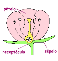
- Load the
irisdata frame (data(iris)), which details the characteristics of 150 flowers across 3 species. Create a scatter plot visualizing the relationship between sepal length and petal length.
- Enhance the previous visualization by coloring the points to represent the species of each flower.
- Polish your plot by setting the title to “Relationship between sepal and petal size of different flowers”, naming the x-axis “Sepal length (in cm)”, the y-axis “Petal length (in cm)”, and labeling the legend simply as “Species”.
Solution
- Generate a statistical summary of the ratio between sepal length and petal length, reporting a data frame that includes the average, standard deviation, and median of this ratio.
Solution
- Refine your previous ratio summary to show these statistics (average, standard deviation, and median) calculated separately for each species.
Solution
5.11 Key Takeaways
This chapter emphasized a layered approach to visualization, building plots incrementally with aesthetics, geoms, and scales. We learned to map data to visual properties using aes, select the appropriate geometry (like geom_point or geom_line), and transform axes to reveal patterns in skewed data. Beyond the visuals, we explored how to customize themes and labels for clarity, and how to quantify insights using dplyr summarization tools before saving our work with ggsave().
What is the standard deviation?↩︎