Chapter 7 Discrete Probabilities
We will start with some basic principles of categorical data. Probabilities of this type are called discrete probabilities. Understanding the basic principles of discrete probabilities will help us understand continuous probabilities which are the most common in data science applications.
In this chapter, we will master the foundations of discrete probability. We will start by calculating probabilities using mathematical definitions and then learn to estimate them using Monte Carlo simulations. We will leverage R functions like sample(), replicate(), and mean() to model random events, and use the gtools package to solve problems involving permutations and combinations. Finally, we will determine how to choose an adequate sample size to ensure our simulations yield reliable results.
Recall that a discrete variable is a variable that cannot take some values within a minimum countable set, that is, it does not accept any value, only those that belong to the set.
For example, if we have 4 women and 6 men seated in a room and we were to raffle 1 prize, intuitively we would know that the probability that the winner is a man is 60%.
7.1 Calculation using the mathematical definition
The probability we obtained by intuition in the previous example can be expressed as follows:
\(P(A) = probability\ of\ event\ A = \frac{Times\ event\ A\ can\ occur}{Total\ possible\ outcomes}\)
\(P(Winner\ is\ man) = \frac{6}{10} = 60\%\)
7.2 Monte Carlo Simulation for Discrete Variables
Monte Carlo simulation or method is a statistical method used to solve complex mathematical problems through the generation of random variables. In this case the problem is not complex, but Monte Carlo can be used to familiarize ourselves with a method that we will use constantly.
We will use Monte Carlo simulation to estimate the proportion we would obtain if we repeated this experiment randomly a determined number of times. That is, the probability of the event using this estimation would be the proportion of times that event occurred in our simulation.
In R we can easily create random samples using the sample() function. For example, let’s create a vector of students and then use the sample() function to choose one at random.
students <- c("woman", "woman", "woman", "woman", "man",
                 "man", "man", "man", "man", "man")

sample(students, 1)
We could also use the rep() function to create the students vector faster. To do this we would enter as the first argument a vector and as the second another vector indicating how many times we want them to be created. Thus, we would create the students vector faster.
students <- rep(c("woman", "man"), times = c(4, 6))

students
#>  [1] "woman" "woman" "woman" "woman" "man"   "man"   "man"   "man"   "man"
#> [10] "man"
Now we have to simulate a determined number of times the experiment of picking a random element. For this we will use the replicate() function. Let’s replicate this experiment 100 times:
students <- rep(c("woman", "man"), times = c(4, 6))

n_times <- 100

results <- replicate(n_times, {
  sample(students, 1)
  })

results
#>   [1] "man"   "man"   "woman" "man"   "man"   "woman" "man"   "woman" "man"
#>  [10] "woman" "man"   "man"   "woman" "man"   "man"   "man"   "woman" "woman"
#>  [19] "woman" "man"   "man"   "man"   "man"   "man"   "man"   "woman" "man"
#>  [28] "woman" "man"   "man"   "man"   "man"   "man"   "woman" "man"   "man"
#>  [37] "man"   "man"   "woman" "man"   "man"   "man"   "man"   "woman" "man"
#>  [46] "woman" "man"   "man"   "woman" "man"   "man"   "woman" "woman" "woman"
#>  [55] "man"   "woman" "man"   "woman" "man"   "man"   "woman" "woman" "woman"
#>  [64] "man"   "man"   "man"   "man"   "man"   "man"   "man"   "man"   "man"
#>  [73] "man"   "woman" "man"   "man"   "man"   "woman" "man"   "man"   "woman"
#>  [82] "woman" "woman" "man"   "woman" "man"   "man"   "man"   "woman" "woman"
#>  [91] "man"   "man"   "man"   "woman" "man"   "woman" "woman" "man"   "man"
#> [100] "man"
We can see what the result was for each of the 100 draws we simulated.
Now we will use the table() function to transform our results vector into a summary table that shows us how many times each value appeared.
If we store this result in a vector results_table, we can then use the prop.table() function to know the proportion of each value:
We should not worry if the probability that it is a man has not come out exactly 60%. Recall that we are estimating the probability using a method that depends on the number of times we simulate the experiment. The more times we repeat the experiment the closer we will be to the value. For example, let’s replicate this experiment now 10,000 times.
students <- rep(c("woman", "man"), times = c(4, 6))

n_times <- 10000

results <- replicate(n_times, {

  sample(students, 1)

  })

results_table <- table(results)

prop.table(results_table)
#> results
#>    man  woman
#> 0.5932 0.4068
We see how the value converges to 60%. We should not worry if the value varies by a few digits from the one presented in this book given that we are simulating a random event.
Finally, for this simple example we could also have used the mean() function. Although this calculates the average of a set of numbers, we could convert our students vector to numerical values, where each value is converted to 1 or 0 depending on some condition.
To do this, R makes the conversion of vectors to 1 and 0 very simple using the comparator operator ==:
When we apply the mean() function to this result, it coerces TRUE values to 1 and FALSE values to 0. Thus, if we apply the average of this list, we would have the percentage of men and with it the probability that when choosing a person it is a man:
7.2.1 Other functions to create vectors
We have already learned the rep() function to create vectors faster. Another function we find in R is the expand.grid(x, y) function which creates a data frame of all combinations between vectors x and y.
greetings <- c("Hello", "Goodbye")
names_list <- c("Andrew", "Joseph", "John", "Emily", "Cesar", "Jeremy")

result <- expand.grid(greeting = greetings, name = names_list)
result
#>    greeting   name
#> 1     Hello Andrew
#> 2   Goodbye Andrew
#> 3     Hello Joseph
#> 4   Goodbye Joseph
#> 5     Hello   John
#> 6   Goodbye   John
#> 7     Hello  Emily
#> 8   Goodbye  Emily
#> 9     Hello  Cesar
#> 10  Goodbye  Cesar
#> 11    Hello Jeremy
#> 12  Goodbye Jeremy
Finally, we have the paste(x,y) function, which concatenates two strings or vectors of strings adding a space in the middle.
paste(result$greeting, result$name)
#>  [1] "Hello Andrew"   "Goodbye Andrew" "Hello Joseph"   "Goodbye Joseph"
#>  [5] "Hello John"     "Goodbye John"   "Hello Emily"    "Goodbye Emily"
#>  [9] "Hello Cesar"    "Goodbye Cesar"  "Hello Jeremy"   "Goodbye Jeremy"
Thus, we can easily generate, for example, a deck of cards distributed in 4 suits: hearts, diamonds, spades, and clubs. The cards of each suit are numbered from 1 to 10, where 1 is the Ace, and followed by Jack, Queen, and King.
To do this, we would have to create a vector of suits and a vector of numbers to then create the combinationl and have the complete deck.
numbers <- c("Ace", "Two", "Three", "Four", "Five", "Six", "Seven",
             "Eight", "Nine", "Ten", "Jack", "Queen", "King")
suits <- c("of Hearts", "of Diamonds", "of Spades", "of Clubs")

# Create card combinations
combination <- expand.grid(number = numbers, suit = suits)

# Concatenate vectors to have our final combination
paste(combination$number, combination$suit)
#>  [1] "Ace of Hearts"     "Two of Hearts"     "Three of Hearts"
#>  [4] "Four of Hearts"    "Five of Hearts"    "Six of Hearts"
#>  [7] "Seven of Hearts"   "Eight of Hearts"   "Nine of Hearts"
#> [10] "Ten of Hearts"     "Jack of Hearts"    "Queen of Hearts"
#> [13] "King of Hearts"    "Ace of Diamonds"   "Two of Diamonds"
#> [16] "Three of Diamonds" "Four of Diamonds"  "Five of Diamonds"
#> [19] "Six of Diamonds"   "Seven of Diamonds" "Eight of Diamonds"
#> [22] "Nine of Diamonds"  "Ten of Diamonds"   "Jack of Diamonds"
#> [25] "Queen of Diamonds" "King of Diamonds"  "Ace of Spades"
#> [28] "Two of Spades"     "Three of Spades"   "Four of Spades"
#> [31] "Five of Spades"    "Six of Spades"     "Seven of Spades"
#> [34] "Eight of Spades"   "Nine of Spades"    "Ten of Spades"
#> [37] "Jack of Spades"    "Queen of Spades"   "King of Spades"
#> [40] "Ace of Clubs"      "Two of Clubs"      "Three of Clubs"
#> [43] "Four of Clubs"     "Five of Clubs"     "Six of Clubs"
#> [46] "Seven of Clubs"    "Eight of Clubs"    "Nine of Clubs"
#> [49] "Ten of Clubs"      "Jack of Clubs"     "Queen of Clubs"
#> [52] "King of Clubs"
Once our deck is created we can inquire some probabilities easily with the created vector.
Let’s calculate the probability that when choosing a card it is “King of Diamonds”:
# Store the combinationl in the variable deck
deck <- paste(combination$number, combination$suit)

mean(deck == "King of Diamonds")
#> [1] 0.01923077
Or we can also calculate the probability that when choosing a card it is some Queen:
# First create the vector of "Queen of..."
queens <- paste("Queen", suits)

# Probability calculation
mean(deck %in% queens)
#> [1] 0.07692308
This chapter highlighted two complementary approaches to probability. The mathematical definition (\(P(A) = \frac{\text{favorable outcomes}}{\text{total outcomes}}\)) gives us exact answers for simple problems. However, for more complex scenarios, Monte Carlo simulation allows us to estimate probabilities by replicating experiments thousands of times using sample() and replicate(). We learned that mean(condition) is an efficient way to calculate proportions in R, and that increasing the number of repetitions brings our simulation estimates closer to the true theoretical probability.
7.3 Exercises
- Calculate the probability of not rolling a 1 on a single die roll and store it in a variable named
prob. Then, use this variable to determine the probability that the number 1 does not appear in three consecutive rolls.
- Imagine a container holding 5 blue, 3 yellow, and 4 gray marbles. Determine the probability that a marble chosen at random is blue.

Solution
marbles <- rep(c("blue", "yellow", "gray"), times = c(5, 3, 4))

# Solution using monte carlo simulation, repeating the event 10,000 times:
results <- replicate(10000, {

  sample(marbles, 1)

  })

prop.table(table(results))

# Solution using the `mean()` function:
mean(marbles == "blue")
Mathematically it would be:
Given the event: \(X = chosen\ marble\ is\ blue\):
\(P(X)=\frac{5}{5+3+4}=\frac{5}{12}=41.67\%\)
The probability that the marble is blue is 41.67%.
- Using the same container of marbles, calculate the probability that a randomly chosen marble is not blue.
Solution
The probability is 58.33%.
Mathematically it would be:
Given the event \(X = chosen\ marble\ is\ blue\):
\(P(\sim~X)=1-P(X)=1-\frac{5}{12}=1-41.67\%=58.33\%\)
- Consider drawing two marbles from the container in sequence without replacing the first one. Calculate the probability that the first marble is blue and the second is not blue. Create numeric variables for each color count to perform this calculation.
Solution
# Create variables
blue <- 5
yellow <- 3
gray <- 4

# Calculate probability that the first marble is blue:
p_1 <- blue / (blue + yellow + gray)

# First calculate the probability that the second is blue:
p_aux <- (blue - 1) / (blue - 1 + yellow + gray)

# Calculate the complement because they ask that the second is NOT blue:
p_2 <- 1 - p_aux

# Calculate what is asked:
p_1 * p_2
This is called sampling without replacement. We have two events, we are taking out two marbles. The second event depends on the first. These two events are not independent of each other.
- Repeat the previous experiment, but this time replace the first marble before drawing the second one. Update your R code to calculate the probability that the first marble is blue and the second is not blue under these conditions.
Solution
# Create variables
blue <- 5
yellow <- 3
gray <- 4

# Calculate probability that the first marble is blue:
p_1 <- blue / (blue + yellow + gray)

# First calculate the probability that the second is blue:
p_aux <- blue / (blue + yellow + gray)

# Calculate the complement because they ask that the second is NOT blue:
p_2 <- 1 - p_aux

# Calculate what is asked:
p_1 * p_2
This is called sampling with replacement. We have two events, we are taking out two marbles again. The second event does not depend on the first. These two events are independent.
7.4 Combinations and Permutations
Some probability situations involve multiple events. When one of the events affects others, they are called dependent events. For example, when objects are chosen from a list or group and are not returned, the first choice reduces the options for future choices.
There are two ways to order or combine results of dependent events. Permutations are groupings in which the order of objects matters. Combinations are groupings in which the content matters but the order does not.
For this we will use the gtools package, which includes libraries like gtools that provide us with intuitive functionalities to work with permutations and combinations.
# First install the gtools package
install.packages("gtools")

# To start using it, load the gtools library
library(gtools)
7.4.1 Permutations
The order matters when we calculate, for example, the winners of a competition. Suppose we have 10 students who are competing on equal terms for who builds the most accurate machine learning model.
data_scientists <- c("Jenny", "Freddy", "Yasan", "Iver", "Pamela", "Alexandra",
                     "Bladimir", "Enrique", "Karen", "Christiam")
Only the top 3 will receive the prize. In this case the order matters, so we will use the function permutations(total, selection, data) where total indicates the size of the vector, selection indicates the size of the result I want, and finally data is my source vector.
We have already calculated all possible results. We can calculate on this result the probability that Freddy wins the competition and that Pamela is in second place.
7.4.2 Combinations
The order does not matter when, for example, we form groups of 2 to participate in the competition.
If now only one team is going to win the prize, we could calculate the probability that the team made up of Pamela and Enrique are the ones who win.
results <- combinations(10, 2, v = data_scientists)

# Total results:
nrow(results)
#> [1] 45

# Probability:
mean((results[, 1] == "Pamela" & results[, 2] == "Enrique") |
     (results[, 1] == "Enrique" & results[, 2] == "Pamela"))
#> [1] 0.02222222
Although we can obtain the probability by calculating all combinations, in R it will be very frequent to use Monte Carlo to estimate the probability by simulation. For the previous case we would not have to generate all combinations, but simply take a sample of two people who would be the members of the winning team. Recall that we have assumed that everyone has equal chances of winning.
Then, we would have to replicate this experiment over and over again, store the sampling results and calculate the proportion of how many times the winning team was composed of Pamela and Enrique.
n <- 10000

result <- replicate(n, {
      team <- sample(data_scientists, 2)

      meets_condition <- (team[1] == "Pamela" & team[2] == "Enrique") |
                          (team[2] == "Pamela" & team[1] == "Enrique")

      meets_condition
})

mean(result)
#> [1] 0.0216
Note that, as we saw previously, the value converges as we increase the number of times we repeat the experiment n. We have simulated repeating the experiment 10 thousand times. However, how many times would it be necessary to replicate the experiment to trust the results of the simulation?
7.5 Sufficient Experiments with Monte Carlo Simulation
Intuitively we can indicate that the greater the number of experiments the more precise the estimated probability. We can, thus, do several simulations with different number of experiments for each simulation. In this way we could find a reasonable number of experiments for our simulation. To do this, first we create a numerical vector where the number of times we are going to simulate the experiment is indicated. Our vector will contain the following values: 10, 20, 40, 80, 160,…, etc. This means that the first time we will simulate the experiment 10 times, the second 20 times and so on.
n_times <- 10*2^(1:17)
n_times
#>  [1]      20      40      80     160     320     640    1280    2560    5120
#> [10]   10240   20480   40960   81920  163840  327680  655360 1310720
Then, we use the code we created to replicate the experiment to create a function called probability_by_sample:
probability_by_sample <- function(n) {
  result <- replicate(n, {
    team <- sample(data_scientists, 2)

    meets_condition <- (team[1] == "Pamela" & team[2] == "Enrique") |
                        (team[2] == "Pamela" & team[1] == "Enrique")

    meets_condition
  })

  mean(result)
}
We already have a function that allows us to replicate the experiment as many times as we want. For example, in the previous section we simulated 10 thousand experiments. Now that we have created the function we would do:
Again, this is a simulation. So every time we execute that function the probability will vary as it is a random sample.
To apply a function on each of the values of a vector we use the function sapply(vector, function) where vector is the vector where the data on which I want to apply the function is and function is the function I want to apply.
prob <- sapply(n_times, probability_by_sample)

prob
#>  [1] 0.00000000 0.00000000 0.00000000 0.02500000 0.02187500 0.01406250
#>  [7] 0.02031250 0.02226563 0.02167969 0.02353516 0.02358398 0.02136230
#> [13] 0.02254639 0.02181396 0.02215576 0.02211456 0.02224197
This gives us the probabilities depending on the number of times we repeat the experiment. Now let’s place these results in a scatter plot to see how it converges
probabilities <- data.frame(
  n = n_times,
  probability = prob
)

probabilities |>
  ggplot() +
  aes(n, probability) +
  geom_line() +
  geom_point() +
  xlab("# of times of the experiment")
We can also change the scale to zoom in on the probabilities for smaller experiment number values and add a reference line with the theoretical probability value calculated previously:
probabilities |>
  ggplot() +
  aes(n, probability) +
  geom_line() +
  geom_point() +
  xlab("# of times of the experiment") +
  scale_x_continuous(trans = "log2") +
  geom_hline(yintercept = 0.022222, color = "blue", lty = 2)
We observe that, for this experiment, repeating the experiment 10 thousand times (x-axis = 3 because it is \(10^3\)) already gives us a good approximation to the real value.
7.6 Case: Birthdays in Classrooms
Let’s review the concepts learned with another example. In a Data Science for Managers class there are 50 students. Using Monte Carlo simulation, let’s estimate what is the probability that there are at least two people who have birthdays on the same day. (Let’s ignore those who have birthdays on February 29).
First let’s list all the days of the year available for birthdays:
Let’s generate a random sample of 50 numbers from the days vector, but this time with replacement because a person could have the same day, and store it in the colleagues variable.
To validate if any of the values are repeated we will use the duplicated() function which validates if there are duplicate values within the vector:
duplicated(colleagues)
#>  [1] FALSE FALSE FALSE FALSE FALSE FALSE FALSE FALSE FALSE FALSE FALSE FALSE
#> [13] FALSE FALSE FALSE FALSE FALSE FALSE FALSE FALSE FALSE FALSE FALSE FALSE
#> [25] FALSE FALSE FALSE FALSE FALSE  TRUE FALSE FALSE FALSE FALSE FALSE FALSE
#> [37] FALSE FALSE FALSE FALSE FALSE  TRUE FALSE FALSE FALSE FALSE FALSE FALSE
#> [49] FALSE FALSE
Finally, to determine if there was any TRUE value we use the any() function:
The result tells us whether it is true or not that there are at least two people who have birthdays on the same day. To estimate by Monte Carlo simulation what the probability is, we have to repeat the experiment many times and take the proportion of how many times we get TRUE as a result.
# Monte Carlo simulation with 10 thousand repetitions
n_times <- 10000

results <- replicate(n_times, {

    colleagues <- sample(days, 50, replace = TRUE)

    # Returns a logical value of whether there are duplicates
    any(duplicated(colleagues))
})

# Probability:
mean(results)
#> [1] 0.9708
We see that the estimated probability is very high, above 95%. What would happen if I have a room of 25 people?
To do this, we modify the previous code and create the variable classroom which will indicate the number of students in that class:
# Monte Carlo simulation with 10 thousand repetitions
n_times <- 10000
classroom <- 25

results <- replicate(n_times, {    # Returns a logical vector
    colleagues <- sample(days, classroom, replace = TRUE)
    any(duplicated(colleagues))
})

# Probability:
mean(results)
#> [1] 0.5668
Let’s now create the function estimate_probability and estimate using this function the probability of finding at least two people with the same birthday in a room of 25 people. This time we have to specify that the sampling is with “replacement” because by default the sample() function is “without replacement”.
# Create the function
estimate_probability <- function(classroom, n_times = 10000){
    results <- replicate(n_times, {    # Returns a logical vector
        colleagues <- sample(days, classroom, replace = TRUE)
        any(duplicated(colleagues))
    })

    # Probability:
    mean(results)
}

estimate_probability(25)
#> [1] 0.5787
Finally, if we already have a function that calculates based on the number of people in a room we can create a numerical vector with the total number of people from different rooms and then apply the function we have created. The result can be stored in the variable prob.
# Create 80 different classrooms
# The first room with 1 person, the last room with 80 people
classrooms <- 1:80

# Estimate probability depending on the number of students per room
prob <- sapply(classrooms, estimate_probability)

prob
#>  [1] 0.0000 0.0020 0.0066 0.0185 0.0251 0.0432 0.0577 0.0747 0.0984 0.1161
#> [11] 0.1384 0.1772 0.1950 0.2217 0.2562 0.2871 0.3164 0.3433 0.3835 0.4133
#> [21] 0.4371 0.4761 0.4993 0.5415 0.5738 0.5962 0.6262 0.6519 0.6784 0.7067
#> [31] 0.7279 0.7451 0.7805 0.7913 0.8211 0.8382 0.8458 0.8642 0.8801 0.8971
#> [41] 0.9017 0.9143 0.9257 0.9347 0.9420 0.9490 0.9536 0.9617 0.9679 0.9703
#> [51] 0.9773 0.9788 0.9819 0.9827 0.9874 0.9884 0.9886 0.9914 0.9938 0.9948
#> [61] 0.9948 0.9961 0.9958 0.9964 0.9974 0.9979 0.9989 0.9990 0.9987 0.9991
#> [71] 0.9993 0.9992 0.9995 0.9996 0.9997 1.0000 0.9997 0.9998 1.0000 0.9999
Thus, if we place it in a scatter plot we can see how the probability increases as there are more students:
probabilities <- data.frame(
  n = classrooms,
  probability = prob
)

probabilities |>
  ggplot() +
  aes(n, probability) +
  geom_point() +
  xlab("Number of students in each class")
We can now impress our friends from different groups by telling them that, if they are in a room of 60 people, “you can bet them” that there are two people in that room who have birthdays on the same day. It is not definitive, but the chances are very much in our favor.
7.7 Exercises
- Alonso and Georgina play chess, and Georgina has a 60% chance of winning any given game. Without using a simulation, calculate the probability that Alonso wins at least one game out of four played.
Solution
Calculating the probability that Alonso has won at least once is the complement of the probability that Georgina has won all 4 times. Thus, we will first calculate the probability that Georgina has always won and then calculate the complement.
- Now, estimate the probability of Alonso winning at least one of four games using a Monte Carlo simulation. Assume Alonso has a 40% chance of winning each individual match.
Solution
- Generalize the previous simulation by creating a function
probability_of_winningthat accepts Alonso’s win probabilitypas an argument. Use this function to simulate outcomes for a sequence of win probabilities from 0.4 to 0.95 (steps of 0.025) and visualize the results in a scatter plot.
Solution
# Create function
probability_of_winning <- function(p){
  n_times <- 10000

  alonso_wins <- replicate(n_times, {
      game_results <- sample(c("loses","wins"), 4, replace = TRUE, prob = c(1-p, p))
      any(game_results == "wins")
  })

  mean(alonso_wins)

}

# Create vector with different probabilities
p <- seq(0.4, 0.95, 0.025)

prob <- sapply(p, probability_of_winning)

plot(p, prob, xlab="p: probability that Alonso wins in each game",
     ylab="prob: prob. that Alonso wins at least one game")
7.8 Integrative Exercise
Let’s solve together this exercise that integrates everything we have learned in this chapter, called the Monty Hall problem.
7.8.1 Monty Hall Problem
Monty Hall was a TV presenter who made famous a contest in his show which we are going to replicate below. We have three doors in front of us:
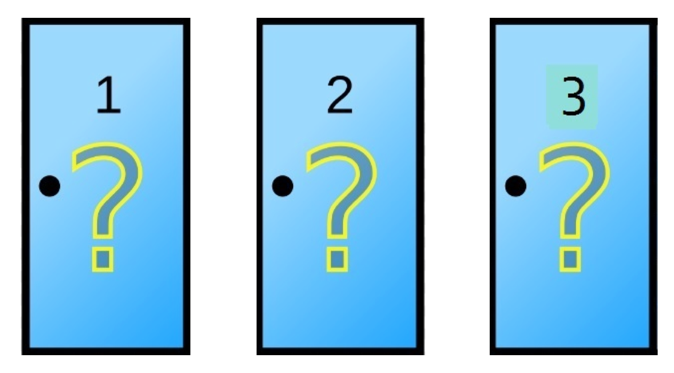
Behind one of these doors is a zero-kilometer car, while in the other two there is a goat. We, as contest participants, have to choose together which door to open. Whatever is behind it will be ours.
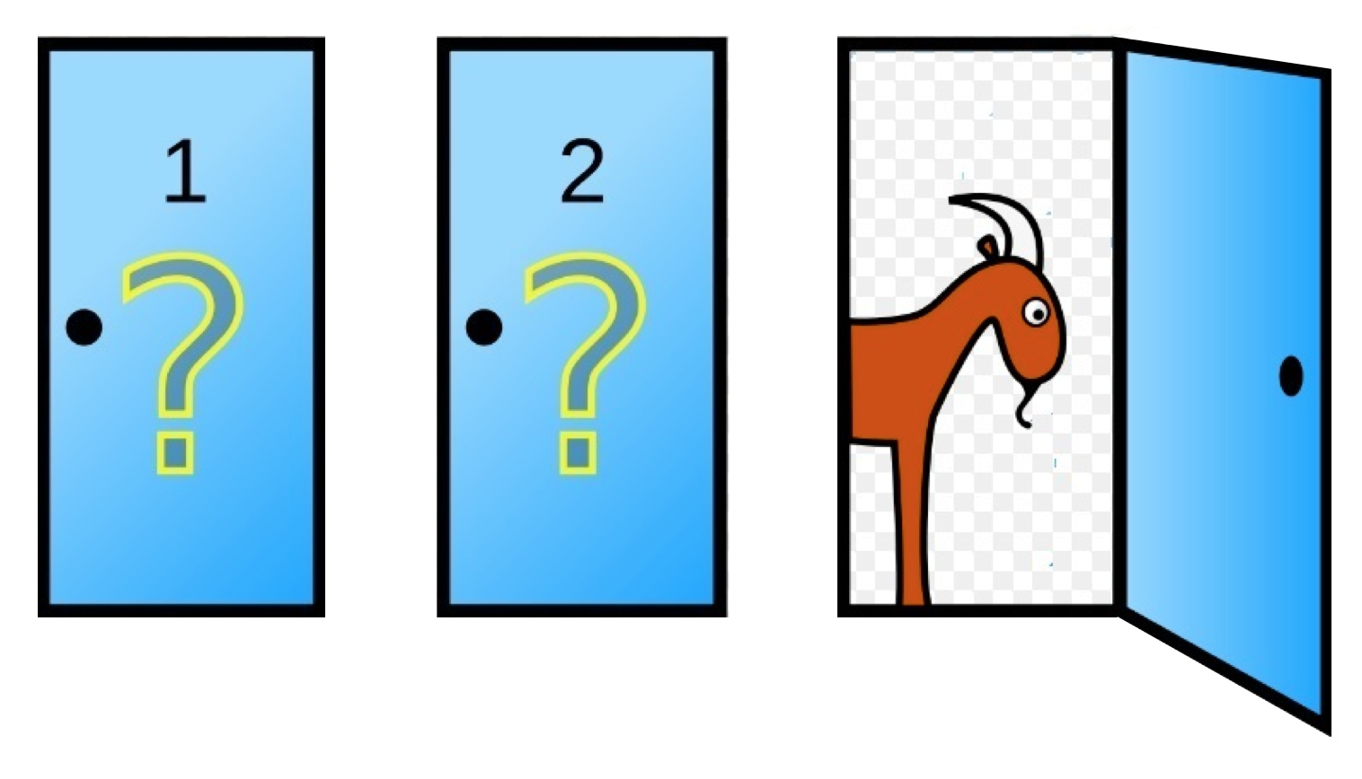
Suppose we have chosen door number 2. Once you announce our choice, Monty Hall tells us that he is going to help us and opens a door for us right now. He opens one of the other doors and it turns out there is a goat in door 3 that he opened.
Monty Hall asks us:
I am going to give you a chance to change doors and that will be your final choice, Would you change doors or stick with the door chosen at the beginning?
Intuitively we knew that, when all doors were closed, the car is in one of 3 doors. The probability of winning would be \(\frac{1}{3} = 0.3333\) so it didn’t matter which door to choose. But when he opens door number three he gives us information and the first thing we should ask ourselves is whether the probabilities have been affected or not. Although this is an advanced math exercise using change of variable, we can execute a Monte Carlo simulation to estimate the probabilities and solve it without using almost any mathematical formula.
Let’s start by simulating the experiment. At the beginning we had three doors, door 1, 2 and 3. We will create the variable doors.
Then, we know that behind the doors there is a car and two goats distributed randomly. We will use the function sample to order them randomly.
Since Monty Hall knows where the prize is. We are going to create a variable prize_door where we will store where the car is.
Now we choose a door randomly and store our result in the variable choice.
Given that we already have the chosen door shown we will simulate Monty Hall choosing the door to open. Since he is the presenter he will choose any door that is not the door where the prize is or your door.
Finally, we are going to put all the code together and in the last line add the comparison of whether the prize door matches our choice. This time we are going to choose not to change doors, so our choice does not vary.
doors <- c("door 1", "door 2", "door 3")
prizes <- sample(c("car", "goat", "goat"))
prize_door <- doors[prizes == "car"]
choice <- sample(doors, 1)
door_opened <- sample(doors[!doors %in% c(choice, prize_door)],1)

choice == prize_door
With our experiment created we are going to simulate what would happen if we stick with the choice and what would happen if we change it.
7.8.1.1 Stick with the chosen door
Let’s replicate about 10 thousand times to see the proportion of times we would win if we stick with our door.
n_times <- 10000

results <- replicate(n_times, {
      doors <- c("door 1", "door 2", "door 3")
      prizes <- sample(c("car", "goat", "goat"))
      prize_door <- doors[prizes == "car"]
      choice <- sample(doors, 1)
      door_opened <- sample(doors[!doors %in% c(choice, prize_door)],1)

      choice == prize_door
})

mean(results)
#> [1] 0.3352
We see that the probability obtained by Monte Carlo simulation is an estimation very close to the probability that we had intuitively calculated. That is, if we keep our choice of the door we chose we have a 33.33% probability of winning.
But, what happens if we change doors? Is the probability of winning the same?
7.8.1.2 Change door
We are going to use the code and modify it by creating the variable new_choice to make the door change.
n_times <- 10000

results <- replicate(n_times, {
      doors <- c("door 1", "door 2", "door 3")
      prizes <- sample(c("car", "goat", "goat"))
      prize_door <- doors[prizes == "car"]
      choice <- sample(doors, 1)
      door_opened <- sample(doors[!doors %in% c(choice, prize_door)],1)

      new_choice <- doors[!doors %in% c(choice, door_opened)]

      new_choice == prize_door
})

mean(results)
#> [1] 0.6686
As we see, changing the door in this show gave us a probability of 66.66% of winning, while keeping our choice only 33.33%.
It may sound counterintuitive, but statistically speaking it is better to change doors instead of trusting our luck and keeping the initial choice.