Chapter 10 Data import and consolidation
10.1 Importing from files
For importing files, whether they are text types or spreadsheets, we need to know where we are going to import the data from.
10.1.1 Working Directory
By default, when we import files, R will search in the working directory. To find out the path of our working directory we will use the getwd() function.
This is the path where we can place our files to load them. If we want to load data from another folder we can change the working directory using setwd().
Note: While
setwd()works, it is generally discouraged in reproducible workflows because it creates absolute paths that break when code is shared or moved. Consider using RStudio Projects combined with theherepackage, which provideshere::here()to construct relative paths that work across different systems.
For practical purposes, we are going to use a file already available in one of the previously installed packages, dslabs, when we analyzed the danger level to decide which US state to travel to. To do this, we can use the system.file() function and determine the path where the dslabs package was installed.
Likewise, we can list the files and folders within that path using the list.files() function.
dslabs_path <- system.file(package="dslabs")
list.files(dslabs_path)
#>  [1] "data"        "DESCRIPTION" "extdata"     "help"        "html"
#>  [6] "INDEX"       "Meta"        "NAMESPACE"   "R"           "script"
The folder we will use is extdata. We can access the path of this folder if we modify the parameters of the system.file() function.
dslabs_path <- system.file("extdata", package="dslabs")
list.files(dslabs_path)
#>  [1] "2010_bigfive_regents.xls"
#>  [2] "calificaciones.csv"
#>  [3] "carbon_emissions.csv"
#>  [4] "fertility-two-countries-example.csv"
#>  [5] "HRlist2.txt"
#>  [6] "life-expectancy-and-fertility-two-countries-example.csv"
#>  [7] "murders.csv"
#>  [8] "olive.csv"
#>  [9] "RD-Mortality-Report_2015-18-180531.pdf"
#> [10] "ssa-death-probability.csv"
The file we will use is murders.csv. To build the complete path of this file we can concatenate the strings or we can also directly use the file.path(path, file_name) function.
Finally, we will copy the file to our working directory with the file.copy(source_path, destination_path) function.
We can validate the copy with the file.exists(file_name) function.
It is recommended to check the documentation of the file manipulation functions.
10.1.2 readr and readxl packages
Now that we have the file in our working directory, we will use functions within the readr and readxl packages to import files into R. Both are included in the tidyverse package that we previously installed.
The functions we will use the most will be read_csv() and read_excel(). The latter supports .xls and .xlsx extensions.
data_df <- read_csv("murders.csv", show_col_types = FALSE)

# Once imported we can remove the file if we wish
file.remove("murders.csv")
#> [1] TRUE
We see how by default it detects the headers in the first row and assigns them a default data type. Let’s now explore our data_df object.
data_df
#> # A tibble: 51 × 5
#>    state                abb   region    population total
#>    <chr>                <chr> <chr>          <dbl> <dbl>
#>  1 Alabama              AL    South        4779736   135
#>  2 Alaska               AK    West          710231    19
#>  3 Arizona              AZ    West         6392017   232
#>  4 Arkansas             AR    South        2915918    93
#>  5 California           CA    West        37253956  1257
#>  6 Colorado             CO    West         5029196    65
#>  7 Connecticut          CT    Northeast    3574097    97
#>  8 Delaware             DE    South         897934    38
#>  9 District of Columbia DC    South         601723    99
#> 10 Florida              FL    South       19687653   669
#> # ℹ 41 more rows
The first thing it indicates is that the object is of type tibble. This object is very similar to a data frame, but with improved features such as, for example, the number of rows and columns in the console, the data type under the header, the default report of only the first 10 records automatically, among many others that we will discover in this chapter.
The same syntax and logic would apply for importing an excel file. In this case we are importing directly from the package path and not from our working directory.
excel_example_path <- file.path(dslabs_path, "2010_bigfive_regents.xls")
data_df_from_excel <- read_excel(excel_example_path)
readr gives us 7 different types of functions for importing flat files:
The readr package provides a versatile suite of functions for importing flat files, each tailored to a specific delimiter or format. The most common is read_csv(), designed for comma-separated values. For tab-separated files, we use read_tsv(), while read_delim() offers a general-purpose solution for files with custom delimiters (like semicolons or pipes). Other specialized functions include read_fwf() for fixed-width files, read_table() for whitespace-separated columns, and read_log() for parsing standard web server logs.
Tip: For files that use semicolons as delimiters (common in European locales), use
read_csv2()orread_delim()withdelim = ";". Also, if you encounter import issues, useproblems(data_df)after importing to diagnose parsing errors.
[!TIP] Clean Column Names: Interpreted data often has column names with spaces or capital letters (e.g., “Customer ID”). We highly recommend piping your data into
janitor::clean_names()immediately after reading it to standardize everything tosnake_case(e.g., “customer_id”).
10.1.3 Importing files from the internet
We have seen how we can enter the full path to load a file directly from another source different from our working directory. In the same way, if we have a file in an internet path we can pass it directly to R since read_csv() and the other readr import functions support URL input as a parameter.
Here we see the import of grades from students of the Data Science with R course.
##### Example 1:
# Historical grades data
url <- "https://dparedesi.github.io/Data-Science-with-R-book/data/student-grades.csv"
grades <- read_csv(url, show_col_types = FALSE)
grades <- grades |>
mutate(total = (P1 + P2 + P3 + P4 + P5 + P6)/30*20)
grades |>
select(P1, P2, P3, P4, P5, total) |>
summary()
#> P1 P2 P3 P4 P5
#> Min. :1.000 Min. :1.00 Min. :4.000 Min. :1.000 Min. :1.000
#> 1st Qu.:3.000 1st Qu.:4.00 1st Qu.:5.000 1st Qu.:5.000 1st Qu.:5.000
#> Median :4.000 Median :5.00 Median :5.000 Median :5.000 Median :5.000
#> Mean :3.762 Mean :4.19 Mean :4.905 Mean :4.571 Mean :4.429
#> 3rd Qu.:5.000 3rd Qu.:5.00 3rd Qu.:5.000 3rd Qu.:5.000 3rd Qu.:5.000
#> Max. :5.000 Max. :5.00 Max. :5.000 Max. :5.000 Max. :5.000
#> total
#> Min. :10.67
#> 1st Qu.:16.67
#> Median :18.67
#> Mean :17.43
#> 3rd Qu.:19.33
#> Max. :20.00From this we could visualize a histogram:

Or we could compare between genders which one has the highest median:
We could also extract updated Covid-19 information.
10.2 Tidy data
Ordered data or tidy data are those obtained from a process called data tidying. It is one of the important cleaning processes during processing of large data or ‘big data’ and is a very used step in Data Science. The main characteristics are that each different observation of that variable has to be in a different row and that each variable you measure has to be in a column (Leek 2015).
As we may have noticed, we have been using tidy data since the first chapters. However, not all our data comes ordered. Most of it comes in what we call wide data or wide data.
For example, we have previously used data from Gapminder. Let’s filter the data from Germany and South Korea to remember how we had our data.
gapminder |>
  filter(country %in% c("South Korea", "Germany")) |>
  head(10)
#>        country year infant_mortality life_expectancy fertility population
#> 1      Germany 1960             34.0           69.26      2.41   73179665
#> 2  South Korea 1960             80.2           53.02      6.16   25074028
#> 3      Germany 1961               NA           69.85      2.44   73686490
#> 4  South Korea 1961             76.1           53.75      5.99   25808542
#> 5      Germany 1962               NA           70.01      2.47   74238494
#> 6  South Korea 1962             72.4           54.51      5.79   26495107
#> 7      Germany 1963               NA           70.10      2.49   74820389
#> 8  South Korea 1963             68.8           55.27      5.57   27143075
#> 9      Germany 1964               NA           70.66      2.49   75410766
#> 10 South Korea 1964             65.3           56.04      5.36   27770874
#>            gdp continent         region
#> 1           NA    Europe Western Europe
#> 2  28928298962      Asia   Eastern Asia
#> 3           NA    Europe Western Europe
#> 4  30356298714      Asia   Eastern Asia
#> 5           NA    Europe Western Europe
#> 6  31102566019      Asia   Eastern Asia
#> 7           NA    Europe Western Europe
#> 8  34067175844      Asia   Eastern Asia
#> 9           NA    Europe Western Europe
#> 10 36643076469      Asia   Eastern Asia
We notice that each row is an observation and each column represents a variable. It is ordered data, tidy data. On the other hand, we can see what the data was like for these two countries if we access the source in the dslabs package.
fertility_path <- file.path(dslabs_path, "fertility-two-countries-example.csv")

wide_data <- read_csv(fertility_path, show_col_types = FALSE)

wide_data
#> # A tibble: 2 × 57
#>   country  `1960` `1961` `1962` `1963` `1964` `1965` `1966` `1967` `1968` `1969`
#>   <chr>     <dbl>  <dbl>  <dbl>  <dbl>  <dbl>  <dbl>  <dbl>  <dbl>  <dbl>  <dbl>
#> 1 Germany    2.41   2.44   2.47   2.49   2.49   2.48   2.44   2.37   2.28   2.17
#> 2 South K…   6.16   5.99   5.79   5.57   5.36   5.16   4.99   4.85   4.73   4.62
#> # ℹ 46 more variables: `1970` <dbl>, `1971` <dbl>, `1972` <dbl>, `1973` <dbl>,
#> #   `1974` <dbl>, `1975` <dbl>, `1976` <dbl>, `1977` <dbl>, `1978` <dbl>,
#> #   `1979` <dbl>, `1980` <dbl>, `1981` <dbl>, `1982` <dbl>, `1983` <dbl>,
#> #   `1984` <dbl>, `1985` <dbl>, `1986` <dbl>, `1987` <dbl>, `1988` <dbl>,
#> #   `1989` <dbl>, `1990` <dbl>, `1991` <dbl>, `1992` <dbl>, `1993` <dbl>,
#> #   `1994` <dbl>, `1995` <dbl>, `1996` <dbl>, `1997` <dbl>, `1998` <dbl>,
#> #   `1999` <dbl>, `2000` <dbl>, `2001` <dbl>, `2002` <dbl>, `2003` <dbl>, …
We see that the original data had two rows, one per country and then each column represented a year. This is what we call wide data or wide data. Normally we will have wide data that we first have to convert to tidy data to later be able to perform our analyses.
10.2.1 Transforming to tidy data
The tidyverse library provides two functions to reshape data between wide and long (tidy) formats. We use pivot_longer() to convert from wide data to tidy data and pivot_wider() to convert from tidy data to wide data.
10.2.1.1 pivot_longer function
Let’s see the utility with the wide_data object that we created in the previous section as a result of importing data from the csv. First apply the pivot_longer() function to explore the conversion that is performed by default.
tidy_data <- wide_data |>
  pivot_longer(cols = -country, names_to = "key", values_to = "value")

tidy_data
#> # A tibble: 112 × 3
#>    country key   value
#>    <chr>   <chr> <dbl>
#>  1 Germany 1960   2.41
#>  2 Germany 1961   2.44
#>  3 Germany 1962   2.47
#>  4 Germany 1963   2.49
#>  5 Germany 1964   2.49
#>  6 Germany 1965   2.48
#>  7 Germany 1966   2.44
#>  8 Germany 1967   2.37
#>  9 Germany 1968   2.28
#> 10 Germany 1969   2.17
#> # ℹ 102 more rows
We see how the pivot_longer() function has collected the columns into two, the names column (“key”) and the values column (“value”). We can change the title of these new columns, for example “year” and “fertility”.
tidy_data <- wide_data |>
  pivot_longer(cols = -country, names_to = "year", values_to = "fertility")

tidy_data
#> # A tibble: 112 × 3
#>    country year  fertility
#>    <chr>   <chr>     <dbl>
#>  1 Germany 1960       2.41
#>  2 Germany 1961       2.44
#>  3 Germany 1962       2.47
#>  4 Germany 1963       2.49
#>  5 Germany 1964       2.49
#>  6 Germany 1965       2.48
#>  7 Germany 1966       2.44
#>  8 Germany 1967       2.37
#>  9 Germany 1968       2.28
#> 10 Germany 1969       2.17
#> # ℹ 102 more rows
We use cols = -country to exclude the country column from being pivoted. By default the column names are collected as text. To convert them to numbers we use the names_transform argument.
tidy_data <- wide_data |>
  pivot_longer(cols = -country, names_to = "year", values_to = "fertility",
               names_transform = list(year = as.integer))

tidy_data
#> # A tibble: 112 × 3
#>    country  year fertility
#>    <chr>   <int>     <dbl>
#>  1 Germany  1960      2.41
#>  2 Germany  1961      2.44
#>  3 Germany  1962      2.47
#>  4 Germany  1963      2.49
#>  5 Germany  1964      2.49
#>  6 Germany  1965      2.48
#>  7 Germany  1966      2.44
#>  8 Germany  1967      2.37
#>  9 Germany  1968      2.28
#> 10 Germany  1969      2.17
#> # ℹ 102 more rows
This data would now be ready to create graphs using ggplot().

10.2.1.2 pivot_wider function
Sometimes, as we will see in the following section, it will be useful to go back from rows to columns. For this we will use the pivot_wider() function, where we specify names_from (the column containing the new column names) and values_from (the column containing the values). Additionally, we can use the : operator to indicate from which column to which column we want to select.
tidy_data |>
  pivot_wider(names_from = year, values_from = fertility) |>
  select(country, `1965`:`1970`)
#> # A tibble: 2 × 7
#>   country     `1965` `1966` `1967` `1968` `1969` `1970`
#>   <chr>        <dbl>  <dbl>  <dbl>  <dbl>  <dbl>  <dbl>
#> 1 Germany       2.48   2.44   2.37   2.28   2.17   2.04
#> 2 South Korea   5.16   4.99   4.85   4.73   4.62   4.53
10.2.2 separate function
In the cases described above we had a situation with relatively ordered data. We only had to do a collection transformation and converted to tidy data. However, the data is not always stored in such an easily interpretable way. Sometimes we have data like this:
path <- file.path(dslabs_path, "life-expectancy-and-fertility-two-countries-example.csv")

data <- read_csv(path, show_col_types = FALSE)

data |>
  select(1:5) #Report first 5 columns
#> # A tibble: 2 × 5
#>   country     `1960_fertility` `1960_life_expectancy` `1961_fertility`
#>   <chr>                  <dbl>                  <dbl>            <dbl>
#> 1 Germany                 2.41                   69.3             2.44
#> 2 South Korea             6.16                   53.0             5.99
#> # ℹ 1 more variable: `1961_life_expectancy` <dbl>
If we apply pivot_longer() directly we would not have our data ordered yet. Let’s see:
data |>
  pivot_longer(cols = -country, names_to = "key_col", values_to = "value_col")
#> # A tibble: 224 × 3
#>    country key_col              value_col
#>    <chr>   <chr>                    <dbl>
#>  1 Germany 1960_fertility            2.41
#>  2 Germany 1960_life_expectancy     69.3
#>  3 Germany 1961_fertility            2.44
#>  4 Germany 1961_life_expectancy     69.8
#>  5 Germany 1962_fertility            2.47
#>  6 Germany 1962_life_expectancy     70.0
#>  7 Germany 1963_fertility            2.49
#>  8 Germany 1963_life_expectancy     70.1
#>  9 Germany 1964_fertility            2.49
#> 10 Germany 1964_life_expectancy     70.7
#> # ℹ 214 more rows
We will use the separate() function to separate a column into multiple columns using a specific separator. In this case our separator would be the character _. Also, we will add the attribute extra="merge" to indicate that if there is more than one separator character, do not separate them and keep them joined.
data |>
  pivot_longer(cols = -country, names_to = "key_col", values_to = "value_col") |>
  separate(key_col, c("year", "other_var"), sep="_", extra = "merge")
#> # A tibble: 224 × 4
#>    country year  other_var       value_col
#>    <chr>   <chr> <chr>               <dbl>
#>  1 Germany 1960  fertility            2.41
#>  2 Germany 1960  life_expectancy     69.3
#>  3 Germany 1961  fertility            2.44
#>  4 Germany 1961  life_expectancy     69.8
#>  5 Germany 1962  fertility            2.47
#>  6 Germany 1962  life_expectancy     70.0
#>  7 Germany 1963  fertility            2.49
#>  8 Germany 1963  life_expectancy     70.1
#>  9 Germany 1964  fertility            2.49
#> 10 Germany 1964  life_expectancy     70.7
#> # ℹ 214 more rows
We already have the year separated, but this data is still not tidy data since there is a row for fertility and a row for life expectancy for each country. We have to pass these values from row to columns. And for that we already learned that we can use the pivot_wider() function
data |>
  pivot_longer(cols = -country, names_to = "key_col", values_to = "value_col") |>
  separate(key_col, c("year", "other_var"), sep="_", extra = "merge") |>
  pivot_wider(names_from = other_var, values_from = value_col)
#> # A tibble: 112 × 4
#>    country year  fertility life_expectancy
#>    <chr>   <chr>     <dbl>           <dbl>
#>  1 Germany 1960       2.41            69.3
#>  2 Germany 1961       2.44            69.8
#>  3 Germany 1962       2.47            70.0
#>  4 Germany 1963       2.49            70.1
#>  5 Germany 1964       2.49            70.7
#>  6 Germany 1965       2.48            70.6
#>  7 Germany 1966       2.44            70.8
#>  8 Germany 1967       2.37            71.0
#>  9 Germany 1968       2.28            70.6
#> 10 Germany 1969       2.17            70.5
#> # ℹ 102 more rows
In other cases, instead of separating a column we will want to join them. In future cases we will see how the unite(column_1, column2) function can also be useful.
10.3 Exercises
- Access the Uber Peru 2010 dataset from this link and attempt to import it into an object named
uber_peru_2010. Pay attention to the delimiters used in the file.
Solution
url <- "https://dparedesi.github.io/Data-Science-with-R-book/data/uber-peru-2010.csv"

# We will use read_csv since it is separated by commas
uber_peru_2010 <- read_csv(url, show_col_types = FALSE)

# Upon importing it we realize it is separated by ";"
uber_peru_2010 |>
  head()

# Therefore we import again using read_delim
uber_peru_2010 <- read_delim("external/uber-peru-2010.csv",
                             delim = ";",
                             col_types = cols(.default = "c")
                             )

uber_peru_2010 |>
head()- Import the SINADEF deaths registry from this source into an object called
deaths. Ensure you handle the file encoding correctly to avoid character issues.
Solution
url <- "https://www.datosabiertos.gob.pe/sites/default/files/sinadef-deaths.csv"
url <- "https://dparedesi.github.io/Data-Science-with-R-book/data/sinadef-deaths.csv"

# We will use read_delim because it is delimited by ";" and not by ","
# Also we change the encoding to avoid error in loading
deaths <- read_delim(url, ";",
local = locale(encoding = "latin1"))- Download the resource file from this link to a temporary location. Validating that the file exists, load the specific sheet named “Deflators” into an object named
data.
Solution
# Store the url
url <- "https://dparedesi.github.io/Data-Science-with-R-book/data/resources-other-idd.xlsx"

# Create a temporary name & path for our file. See: ?tempfile
temp_file <- tempfile()

# Download the file to our temp
download.file(url, temp_file)

# Import the excel
dat <- read_excel(temp_file, sheet = "Deflators")

# Remove the temporary file
file.remove(temp_file)
For the following files run the following code so that you have access to the objects referred to in the problems:
# GDP by countries
url <- "https://dparedesi.github.io/Data-Science-with-R-book/data/gdp.csv"
gdp <- read_csv(url, show_col_types = FALSE)

# Diseases by years by countries
url <- "https://dparedesi.github.io/Data-Science-with-R-book/data/diseases-evolution.csv"
diseases_wide <- read_csv(url, show_col_types = FALSE)

# Number of female mayors
url <- "https://dparedesi.github.io/Data-Science-with-R-book/data/female-mayors.csv"
female_mayors <- read_csv(url, show_col_types = FALSE)

# Evolution of a university
url <- "https://dparedesi.github.io/Data-Science-with-R-book/data/university.csv"
university <- read_csv(url, show_col_types = FALSE)- Examine the structure of the
gdpdataset. Transform it into a tidy format suitable for analysis, and then create a line plot visualizing the evolution of GDP over time for each country.
Solution
- The
diseases_wideobject contains disease counts in a wide format. Reshape this dataframe into a tidy structure where the specific diseases are consolidated into a single column.
Solution
# Solution
diseases_1 <- diseases_wide |>
  pivot_longer(cols = c(-country, -year, -population), names_to = "disease", values_to = "count")

diseases_1

# Alternative solution. Instead of indicating what to omit, we indicate what to take into account
diseases_2 <- diseases_wide |>
  pivot_longer(cols = HepatitisA:Rubella, names_to = "disease", values_to = "count")

diseases_2- Convert the
female_mayorsdataset, which is currently in a long format, into a wide format where the variables are spread across columns.
- The
universitydataset is untidy. Reshape it by first pivoting longer to gather variables, separating the combined variable names, and then pivoting wider to achieve a final tidy structure.
10.4 Joining tables
Regularly we will have data from different sources that we then have to combine to be able to perform our analyses. For this we will learn different groups of functions that will allow us to combine multiple objects.
10.4.1 Join functions
Join functions are the most used in table crossing. To use them we have to make sure we have the dplyr library installed.
This library includes a variety of functions to combine tables.
The dplyr package offers a family of join functions to combine tables based on common keys. The most frequently used is left_join(), which preserves all rows from the first (left) table and appends matching data from the second. Conversely, right_join() keeps all rows from the second table. inner_join() is more restrictive, retaining only the rows that have matching keys in both tables, effectively filtering for the intersection. full_join() does the opposite, keeping all rows from both tables and filling missing values with NA. Finally, filtering joins like semi_join() (keeps rows in the first table that match the second) and anti_join() (keeps rows in the first table that do not match the second) are excellent for data validation and filtering without adding new columns.
To see the join functions with examples we will use the following files:
url_1 <- "https://dparedesi.github.io/Data-Science-with-R-book/data/join-card.csv"
url_2 <- "https://dparedesi.github.io/Data-Science-with-R-book/data/join-customer.csv"

card_data_1 <- read_csv(url_1, col_types = cols(id = col_character()))
customer_data_2 <- read_csv(url_2, col_types = cols(id = col_character()))

card_data_1
#> # A tibble: 6 × 3
#>   id       customer_type card
#>   <chr>    <chr>         <chr>
#> 1 45860518 premium       VISA gold
#> 2 46534312 bronze        Mastercard Black
#> 3 47564535 silver        VISA platinum
#> 4 48987654 bronze        American Express
#> 5 78765434 gold          VISA Signature
#> 6 41346556 premium       Diners Club

customer_data_2
#> # A tibble: 8 × 4
#>   id       first_name last_name mother_last_name
#>   <chr>    <chr>      <chr>     <chr>
#> 1 49321442 Iver       Castro    Rivera
#> 2 47564535 Enrique    Gutierrez Rivasplata
#> 3 48987654 Alexandra  Cupe      Gaspar
#> 4 47542345 Christiam  Olortegui Roca
#> 5 41346556 Karen      Jara      Mory
#> 6 45860518 Hebert     Lopez     Chavez
#> 7 71234321 Jesus      Valle     Mariños
#> 8 73231243 Jenny      Sosa      Sosa
10.4.1.1 Left join
Given two tables with the same identifier (in our case our identifier consists only of a single column: ID), the left join function maintains the information of the first table and completes it with the data that crosses in the second table
left_join(card_data_1, customer_data_2, by = c("id"))
#> # A tibble: 6 × 6
#>   id       customer_type card             first_name last_name mother_last_name
#>   <chr>    <chr>         <chr>            <chr>      <chr>     <chr>
#> 1 45860518 premium       VISA gold        Hebert     Lopez     Chavez
#> 2 46534312 bronze        Mastercard Black <NA>       <NA>      <NA>
#> 3 47564535 silver        VISA platinum    Enrique    Gutierrez Rivasplata
#> 4 48987654 bronze        American Express Alexandra  Cupe      Gaspar
#> 5 78765434 gold          VISA Signature   <NA>       <NA>      <NA>
#> 6 41346556 premium       Diners Club      Karen      Jara      Mory
As we can see, the first three columns are exactly the same as we initially had and to the right of those columns we see the columns of the other table for the values that did cross the data. In this case we are facing a data inconsistency since all customers of card_data_1 should be in customer_data_2. This inconsistency could lead us to have to map the data loss process, etc.
10.4.1.2 Right join
Given two tables with the same identifier, the right join function maintains the information of the second table and completes it with the data that crosses in the first table
right_join(card_data_1, customer_data_2, by = "id")
#> # A tibble: 8 × 6
#>   id       customer_type card             first_name last_name mother_last_name
#>   <chr>    <chr>         <chr>            <chr>      <chr>     <chr>
#> 1 45860518 premium       VISA gold        Hebert     Lopez     Chavez
#> 2 47564535 silver        VISA platinum    Enrique    Gutierrez Rivasplata
#> 3 48987654 bronze        American Express Alexandra  Cupe      Gaspar
#> 4 41346556 premium       Diners Club      Karen      Jara      Mory
#> 5 49321442 <NA>          <NA>             Iver       Castro    Rivera
#> 6 47542345 <NA>          <NA>             Christiam  Olortegui Roca
#> 7 71234321 <NA>          <NA>             Jesus      Valle     Mariños
#> 8 73231243 <NA>          <NA>             Jenny      Sosa      Sosa
The idea is the same as in left_join, only this time the NA are in the first two columns.
10.4.1.3 Inner join
In this case we will only have the intersection of the tables. Only the result of the data that are in both tables will be shown.
inner_join(card_data_1, customer_data_2, by = "id")
#> # A tibble: 4 × 6
#>   id       customer_type card             first_name last_name mother_last_name
#>   <chr>    <chr>         <chr>            <chr>      <chr>     <chr>
#> 1 45860518 premium       VISA gold        Hebert     Lopez     Chavez
#> 2 47564535 silver        VISA platinum    Enrique    Gutierrez Rivasplata
#> 3 48987654 bronze        American Express Alexandra  Cupe      Gaspar
#> 4 41346556 premium       Diners Club      Karen      Jara      Mory
10.4.1.4 Full join
Full join is a total crossing of both. It shows us all the data that are in both the first and the second table.
full_join(card_data_1, customer_data_2, by = "id")
#> # A tibble: 10 × 6
#>    id       customer_type card             first_name last_name mother_last_name
#>    <chr>    <chr>         <chr>            <chr>      <chr>     <chr>
#>  1 45860518 premium       VISA gold        Hebert     Lopez     Chavez
#>  2 46534312 bronze        Mastercard Black <NA>       <NA>      <NA>
#>  3 47564535 silver        VISA platinum    Enrique    Gutierrez Rivasplata
#>  4 48987654 bronze        American Express Alexandra  Cupe      Gaspar
#>  5 78765434 gold          VISA Signature   <NA>       <NA>      <NA>
#>  6 41346556 premium       Diners Club      Karen      Jara      Mory
#>  7 49321442 <NA>          <NA>             Iver       Castro    Rivera
#>  8 47542345 <NA>          <NA>             Christiam  Olortegui Roca
#>  9 71234321 <NA>          <NA>             Jesus      Valle     Mariños
#> 10 73231243 <NA> <NA> Jenny Sosa SosaTip: To join on multiple columns, use a vector:
by = c("col1", "col2"). To join on columns with different names, use named vectors:by = c("left_col" = "right_col").
10.4.1.5 Semi join
The case of the semi join is very similar to left_join with the difference that it only shows us the columns of the first table and eliminates the data that did not manage to cross (what in left_join comes out as NA). Also, none of the columns of table 2 appear. This is like doing a filter requesting the following: show me only the data from table 1 that is also in table 2.
10.4.2 Joining without a common identifier
Likewise, we will have some moments when we need to combine only two objects, without using any type of intersection. For this we will use the bind functions. These functions allow us to put together two vectors or tables either in rows or columns.
10.4.2.1 Union of vectors
If we have two or more vectors of the same size we can create the union of the columns to create a table using the bind_cols() function. Let’s see with an example:
10.4.2.2 Union of tables
In the case of tables the use is the same. Likewise, we can also join the rows of two or more tables. To see its application let’s first create some example tables:
table_1 <- data.frame(
  name = c("Jhasury", "Thomas", "Andres", "Josep"),
  surname = c("Campos", "Gonzales", "Santiago", "Villaverde"),
  address = c("Jr. los campos 471", "Av. Casuarinas 142", NA, "Av. Tupac Amaru 164"),
  phone = c("976567325", "956732587", "961445664", "987786453")
)

table_2 <- data.frame(
  age = c(21, 24, 19, 12),
  sign = c("Aries", "Capricorn", "Sagittarius", "Libra")
)

# Create a table from row 2 to 3 of table_1
table_3 <- table_1[2:3, ]
Once we have our tables let’s proceed to join them. We see that they do not have a common identifier.
result <- bind_cols(table_1, table_2)
result
#>      name    surname             address     phone age        sign
#> 1 Jhasury     Campos  Jr. los campos 471 976567325  21       Aries
#> 2  Thomas   Gonzales  Av. Casuarinas 142 956732587  24   Capricorn
#> 3  Andres   Santiago                <NA> 961445664  19 Sagittarius
#> 4   Josep Villaverde Av. Tupac Amaru 164 987786453  12       Libra
or joining by rows like this:
result <- bind_rows(table_1, table_3)
result
#>      name    surname             address     phone
#> 1 Jhasury     Campos  Jr. los campos 471 976567325
#> 2  Thomas   Gonzales  Av. Casuarinas 142 956732587
#> 3  Andres   Santiago                <NA> 961445664
#> 4   Josep Villaverde Av. Tupac Amaru 164 987786453
#> 5  Thomas   Gonzales  Av. Casuarinas 142 956732587
#> 6  Andres   Santiago                <NA> 961445664
10.5 Web Scraping
Web Scraping is the process of extracting data from a website. We will use it when we need to extract data directly from tables that are presented on websites. For this we will use the rvest library, included in the tidyverse library.
Important: When scraping websites, always respect the site’s
robots.txtfile and terms of service. Avoid making excessive requests that could overload servers. For commercial use, consider whether the data is licensed or requires permission.
The function we will use the most will be read_html() and as an argument we will place the url of the web from where we want to extract the data. We are not talking about a url that downloads a text file but a web page like this:
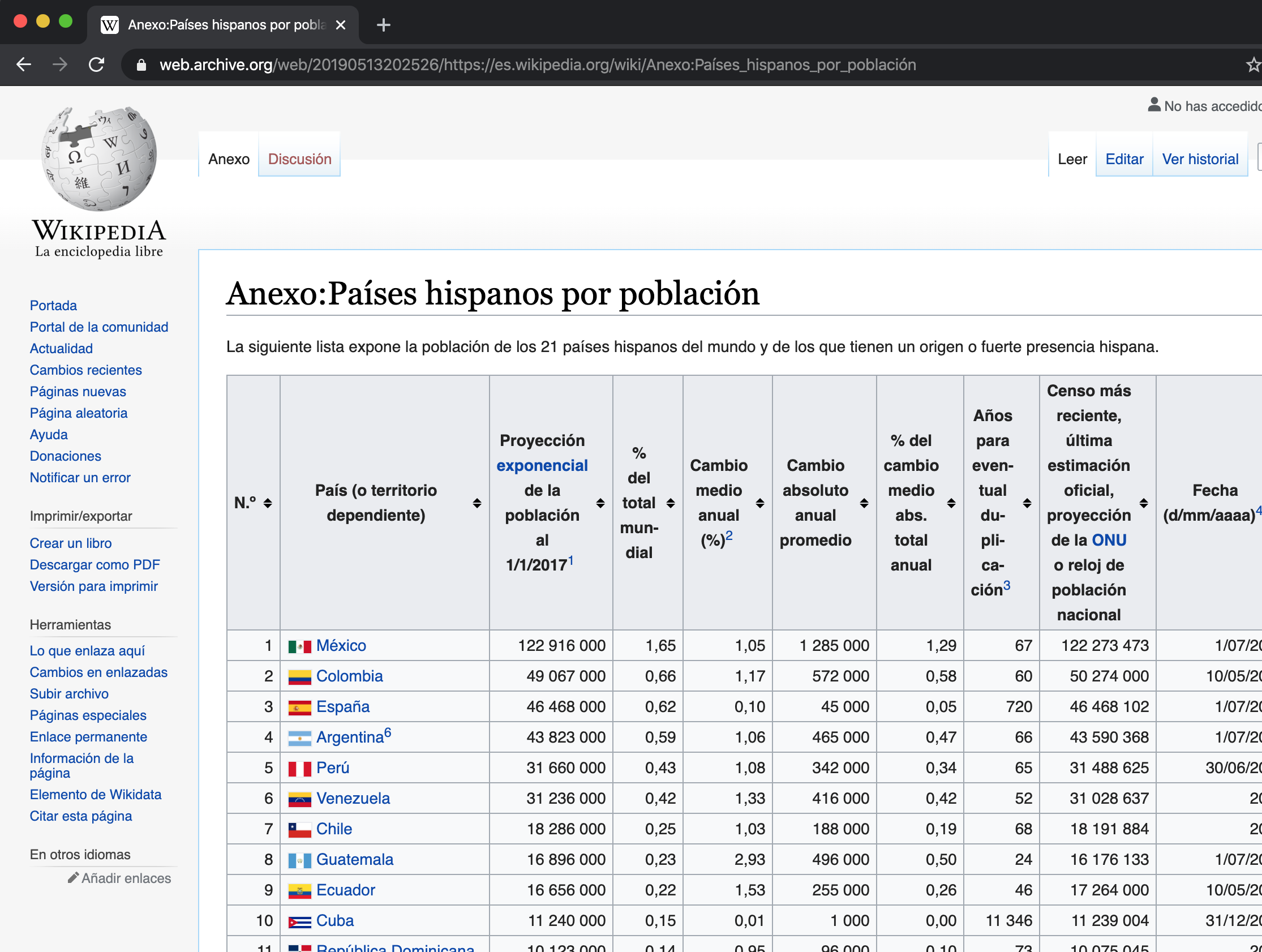
Thus, we will use read_html() to store all the web html and then little by little access the table data in R.
html_data <- read_html("https://es.wikipedia.org/wiki/Anexo:Pa%C3%ADses_hispanos_por_poblaci%C3%B3n")

html_data
#> {html_document}
#> <html class="client-nojs vector-feature-language-in-header-enabled vector-feature-language-in-main-page-header-disabled vector-feature-page-tools-pinned-disabled vector-feature-toc-pinned-clientpref-1 vector-feature-main-menu-pinned-disabled vector-feature-limited-width-clientpref-1 vector-feature-limited-width-content-enabled vector-feature-custom-font-size-clientpref-1 vector-feature-appearance-pinned-clientpref-1 vector-feature-night-mode-enabled skin-theme-clientpref-day vector-sticky-header-enabled vector-toc-available" lang="es" dir="ltr">
#> [1] <head>\n<meta http-equiv="Content-Type" content="text/html; charset=UTF-8 ...
#> [2] <body class="skin--responsive skin-vector skin-vector-search-vue mediawik ...
Now that we have the data stored in the object we have to go looking for the data, doing scraping. For this we will use the html_nodes("table") function to access the “table” node.
Finally, we have to go index by index looking for the table that interests us. To give it table format we will use html_table. In this case we will use double brackets because it is a list of lists and the setNames() function to change the name of the columns.
# We format as table and store in raw_table
raw_table <- web_tables[[1]] |>
  html_table()

# Change header names
raw_table <- raw_table |>
  setNames(
  c("N", "country", "population", "pop_prop", "avg_change", "link")
  )

# Convert to tibble
raw_table <- raw_table |>
  as_tibble()

# Report first rows
raw_table |>
  head(5)
#> # A tibble: 1 × 2
#>   N     country
#>   <lgl> <chr>
#> 1 NA    Este artículo o sección se encuentra desactualizado.La información sumi…
We already have our data imported and we could already start exploring its content in detail.
10.6 Exercises
For the following exercises we will use objects from the Lahman library, which contains US baseball player data. Run the following Script before starting to solve the exercises.
install.packages("Lahman")
library(Lahman)

# Top 10 players of the year 2016
top_players <- Batting |>
  filter(yearID == 2016) |>
  arrange(desc(HR)) |>    # sorted by number of "Home run"
  slice(1:10)    # Take from row 1 to 10

top_players <- top_players |> as_tibble()

# List of all baseball players from recent years
master <- Master |> as_tibble()

# Awards won by players
awards <- AwardsPlayers |>
  filter(yearID == 2016) |>
as_tibble()- Using the
top_playersandMasterdatasets, join them to retrieve theplayerID, first name, last name, and home runs (HR) for the top 10 players of 2016.
Solution
- Identify the intersection of top players and award winners. List the ID and names of the top 10 players from 2016 who also won at least one award that year.
- Find the players who won awards in 2016 but did not make it into the top 10 list. Report their IDs and names.
Solution
# First we calculate all prizes of those who are not top 10:
non_top_award_ids <- anti_join(awards, top_10, by = "playerID") |>
  select(playerID)

# As a player could have obtained several prizes we obtain unique values
non_top_award_ids <- unique(non_top_award_ids)

# Then we cross with the master to obtain the names
other_names <- left_join(non_top_award_ids, master, by = "playerID") |>
  select(playerID, nameFirst, nameLast)

other_names- Scrape the MLB payroll data from
http://www.stevetheump.com/Payrolls.htm. Store the entire page html, extract the tables, and specifically isolate the fourth table (node 4), formatting it as a data frame.
Solution
- Using the scraped tables, prepare the 2019 payroll (node 4) and 2018 payroll (node 5) data. Standardize the column names to
team,payroll_2019, andpayroll_2018respectively. Finally, perform a full join to combine these datasets by team name.
Solution
payroll_2019 <- nodes[[4]] |>
  html_table()

payroll_2018 <- nodes[[5]] |>
  html_table()

####### Payroll 2019: ################
#We eliminate row 15 which is the league average:
payroll_2019 <- payroll_2019[-15, ]

#We filter the requested columns:
payroll_2019 <- payroll_2019 |>
  select(X2, X4) |>
  rename(team = X2, payroll_2019 = X4)

# We eliminate row 1 since it is the source header
payroll_2019 <- payroll_2019[-1,]

####### Payroll 2018: ################
# We select the two columns that interest us and
#change name to headers
payroll_2018 <- payroll_2018 |>
  select(Team, Payroll) |>
  rename(team = Team, payroll_2018 = Payroll)

####### Full join: ################
full_join(payroll_2018, payroll_2019, by = "team")